Fast metaballs
Andreas Jönsson, April 2001
What are metaballs?
One way of describing metaballs is that they are a way of visualizing gravity or energy fields. Take a point in space and measure the energy there. The energy in that point will be the sum of each balls contribution, where the contribution of one ball is higher the closer to that ball the point is. You get the special look of metaballs by rendering a surface that goes through each point in the space that have the energy value of a specified threshold.
Picture of 2d metaballs with several levels of energy.
The needed formulas
The first thing you need is a formula to compute the energy contribution from one ball. This formula should be based on the distance and must be continuous. Preferably it should never get below zero as that will lead to complications later on. Actually it might give a cool effect to have some of the balls give a negative energy contribution, however the algorithm presented in this article will not work with such balls. One perfect candidate for a formula like this is the gravity formula.
g = c m / d2
Where g is the gravity at a certain point, c a constant, m is the mass, and d the distance from the center of mass.
If you want to have some kind of lighting on your metaballs you'll also need a formula for computing the normal in a point in space based on the energy. Some of you might already know that that is simply done by deriving the energy formula, however I suspect some of you don't. I'm a nice guy so I'll give the formula right here so you don't have to do anything.
n = 2 m v / d4
Here n is the normal vector and v is the vector from the center of the ball to the point of interest. One thing to note is that you should only normalize the normal vector after summation of all the parts. This is not only because it is faster but more because you would get the wrong result otherwise.
How to render the metaballs
There are many techniques that can be used for rendering surfaces for this kind of application. If you are interested I suggest you search for techniques for finding iso-surfaces. One of the easier way of doing it is by using a technique called "marching cubes". I'm not going to give a detailed description of how marching cubes work, because there are so many other people that have already done that. If you look at the end of this article you'll find links to some of the better articles that I've found on marching cubes.
In short the marching cubes algorithm can be said to work like this. Take a regular 3D grid of values (volume data). Examine each voxel in this grid to see if the surface goes through it. If it does, compute the vertices by interpolating the values over the edges and render triangles between the vertices.
The cases of marching squares, the 2D brother of marching cubes.
The brute force way of rendering the metaballs would be to compute the energy for every point in the 3D grid and then let marching cubes go through each voxel to compute the surface. This would however be highly inefficient since the metaballs' surface will only go through approximatly 10% of the voxels, perhaps even less.
The algorithm
I will here present an algorithm that computes only the voxels that actually contain the surface, plus a few more to find the surface. I've found this algorithm to be incredibly efficient. I actually managed to create a small demo that has 20 metaballs moving in the scene at the same time, and that was without optimizations. I've previously only seen a maximum of 7 metaballs at the same time, and these most likely used many optimizations, such as efficient assembler code and lookup tables.
RenderMetaballs()
{
  for each ball
  {
    pos = ball's position in the grid
    isComputed = false
    found = false
    while not found
    {
      if voxel is computed
      {
        isComputed = true
        found = true
      }
      else
      {
        case = ComputeVoxel(pos)
        if case < 255
          found = true
        else
          pos = move one step up
      }
    }

    if not isComputed
    {
      AddNeighborsToOpenList(case,pos)
      while open list is not empty
      {
        pos = position of last voxel in open list
        case = ComputeVoxel(pos)
        AddNeighboursToOpenList(case,pos)
      }
    }
  }
}
RenderMetaballs() traces a line from the center of each metaball out until it reaches the surface. If the voxel where the line intersects the surface hasn't been computed yet it will compute that voxel and then progress to the neighbors until all interlinked voxels have been computed. If the voxel has already been computed then this metaball is connected to another, thus the surface doesn't have to be computed again.
ComputeVoxel(pos) uses the marching cubes algorithm to compute the vertices and triangles in this voxel. It then returns the marching cube case so that we can see how the surface lie within the voxel and which neighbors also contain the surface.
AddNeighborsToOpenList(case,pos) adds all neighbors to the list of open voxels unless they have already been added once. It uses the case variable to identify which neighbors actually contain the surface.
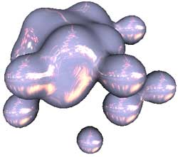
A screenshot from my demo.
A word of warning
The marching cubes algorithm used in this article is a patented algorithm, so make sure you know what you're doing when you use it. For a non-commercial demo you should be quite safe in using this technique but if you plan on using it in a commercial product you might want to investigate into the patent to know just exactly what the patent holder is allowed to do.
Conclusion
I hope that you found this article interesting and perhaps useful. Should you find something that bothers you, perhaps something that you think is an error or just something that's not quite clear then feel free to contact me. I will be happy to discuss it with you.
Thanks to Maciek, a.k.a. Shyha, for pointing out a minor error in the RenderMetaballs() algorithm.